On Dynamic Graph and Edge Convolution Operations

Introduction

This article aims to review and reflect on the EdgeConv operation and DGCNN to develop an understanding of the method and when it is suitable. In fact, while working on the new TopoLineArt architecture (to be published), I began reproducing many GNN operations. DGCNN is an interesting method because it eliminates the need to figure out the relationships between nodes while preparing a graph dataset. Instead, it is sufficient to start with a kNN graph, and the model will then learn how nodes are connected while learning the task (in the case of Wang et al. (2019), the tasks are classification and segmentation).

This case study presents a review of EdgeConv and DGCNN (Wang et al., 2020) and discusses my attempt to reimplement DGCNN using PyTorch Geometric’s EdgeConv operation to classify the 3D objects in the ModelNet10 dataset. In particular, this article aims to reflect on the method and its applicability while walking through and analysing the task and the model’s performance.

Dataset

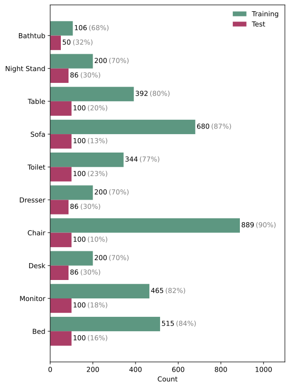
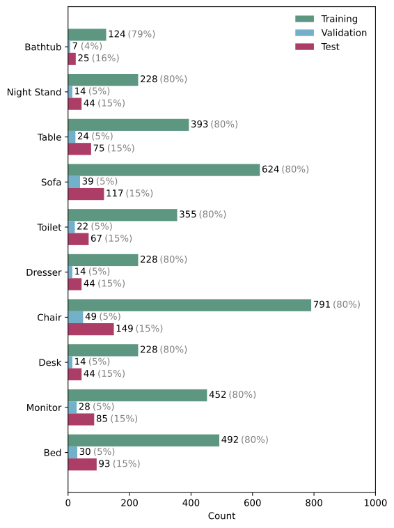
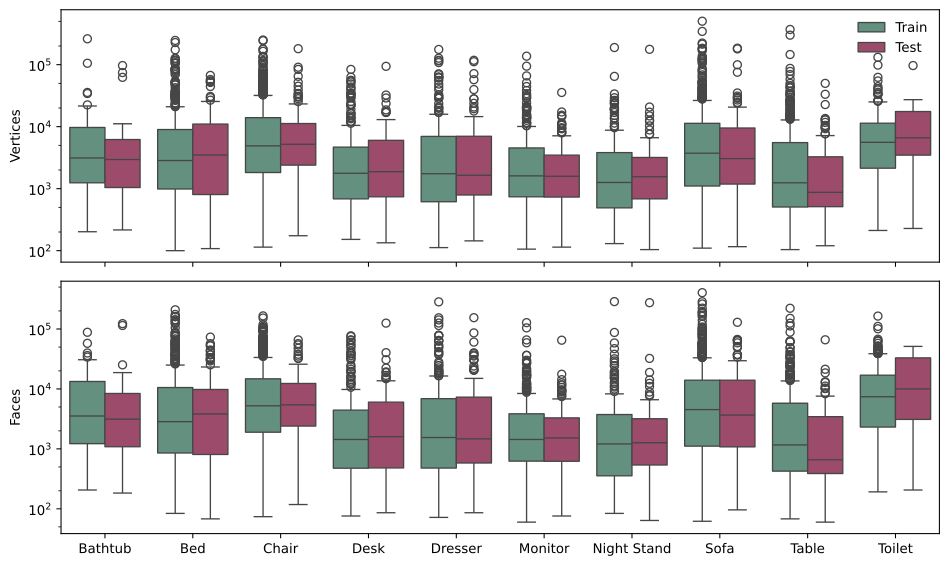
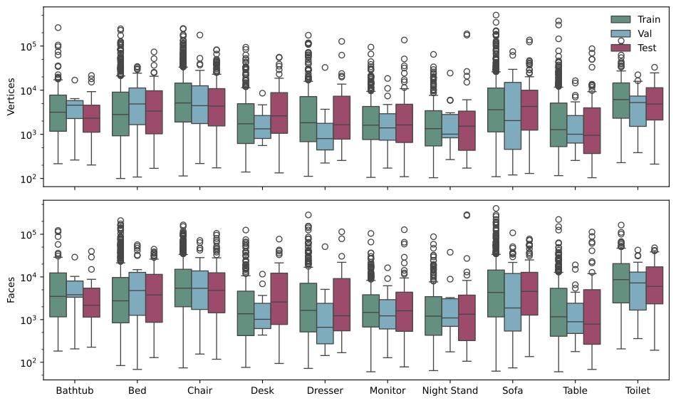
ModelNet10 was the chosen dataset for this case study. This choice was motivated by several factors, including the smaller size of the dataset compared with ModelNet40 (the dataset used in Wang et al. (2020)). The smaller dataset allows for faster training and evaluation and is sufficient for the purposes of this case study. The dataset itself has 4,899 CAD objects saved in Object File Format, which stores information about the faces, vertices, and edges of each object. Out of the box, the dataset has two splits: 3,991 objects for training and 908 for testing. Since the dataset is not split uniformly across classes (Figure 1, left), I resplit the data into training, validation, and test sets using an 80/5/15 ratio (Figure 1, right). Stratified splitting was used to ensure that each class is represented in the same proportion across the training, validation, and test splits, which helps make model training and evaluation more balanced and reliable. The dataset statistics per class before and after resplitting are shown in Figures 2 and 3, respectively.

Class count using the official ModelNet10 train-test split — Figure 1: Class balance in ModelNet10: official split (left) and resplit dataset (right).

Class count after resplitting the ModelNet10 dataset — Figure 1: Class balance in ModelNet10: official split (left) and resplit dataset (right).

The figures below show the distributions of vertex and face counts for each class across the dataset splits. As we can see, these distributions are quite similar across all splits, which means that we can move to the next step and preprocess the data before developing the model. It is worth mentioning that if the distributions of face counts within a single class differed significantly between splits, it would be necessary to investigate further (e.g. by reshuffling the data so that each split has a similar distribution).

Class statistics — Figure 2: Per-class and per-split distributions of the dataset **before** resplitting.

Data Preprocessing and Augmentation

Before the data were passed to the model, points were sampled from the mesh faces, and each shape was normalised to fit inside a unit sphere centred at the origin. The shapes were augmented by rotation around the z-axis (note that rotations around other axes are possible but would place the shapes in awkward orientations that are unlikely to occur in the real world). Additionally, random, uniform, symmetric jitter noise was added to the vertices in the point cloud. Although additional augmentations are possible, such as random scaling or translation, this case study continues to follow the dataset augmentation methods described in the literature being reproduced here.

Method

Graphs, unlike images, have an irregular structure, allowing them to represent arbitrary relationships between nodes. This has allowed for interesting developments in AI for learning on graphs. These methods have proven to be very powerful when data are appropriately represented as graphs. The success of these methods has motivated this case study, along with many other case studies and research projects I am working on.

Baseline: Simplified PointNet

When experimenting with AI (or conducting any experiment in general), it is important to have a baseline that is good enough to compare your model against; otherwise, how can you tell if your model is actually better? I find that, in the early stages of academic research and in case studies like this one, it is sufficient to implement a simplified version of a model from the existing literature. If you later find that comparing your results with those in the existing literature is particularly important, you can implement the full version of the published model once you have a first version of your own model working.

The baseline has three 1D convolutional layers, each with a ReLU activation. The features produced by the final convolution are then aggregated across all points using max pooling. This produces a global feature vector, which is then passed through a fully connected layer, followed by a final classification layer that outputs the logits. Each shape passed to the model had 2048 points and was augmented with jitter noise ( $\sigma = 0.02$ ). The model was trained using the Adam optimiser with a learning rate of $10^{-3}$ for up to 1000 epochs, with an early-stopping patience of 50 epochs.

DGCNN with EdgeConv and PyTorch Geometric

Wang et al. (2019) used a graph representation for each shape’s point cloud. Graphs $\mathcal{G}$ are unordered data structures that are made up of nodes $\mathcal{N}$ and edges $\mathcal{E}$ . The edges model the relationships between nodes, and the graph structure can be expressed as an adjacency matrix. Any function applied to graph data must have one of two important properties:

Permutation Invariance (for graph-level outputs, e.g. graph classification): The function does not care about the order of the nodes (i.e. the rows and columns in the adjacency matrix):

f(PX, PAP^T) = f(X, A)

where $f$ is any function (e.g. a neural network), $A$ is the adjacency matrix, and $P$ is any permutation matrix.

Permutation Equivariance (for node-level outputs, e.g. node classification): If you shuffle the input to a function in some way, its output will be shuffled in the same way; in other words, reordering the nodes causes the corresponding node-level outputs to be reordered in the same way:

F(PX, PAP^T) = P F(X, A)

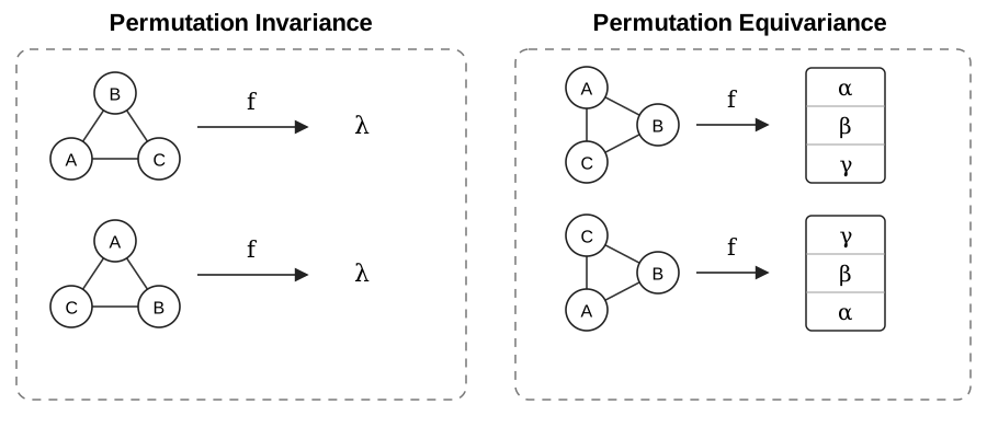
For more details about learning on graphs, feel free to refer to Hamilton (2020) or Bronstein et al. (2021). In their work, Wang et al. (2019) used points as nodes and connected each node to its $k$ nearest neighbours. Edge features are computed as $\mathbf{e}_{ij} = h_\Theta(\mathbf{x}_i, \mathbf{x}_j)$ , where $h_\Theta: \mathbb{R}^F \times \mathbb{R}^F \rightarrow \mathbb{R}^F$ . Here, $F$ is the feature-space dimension, $h$ is a non-linear function, and $\Theta$ denotes its learnable parameters.

The operation used to update node features is called EdgeConv, which is defined by applying the aggregation operation $\square$ to the edge features $\mathbf{e}_{ij}$ associated with all edges linked to a node:

\mathbf{x^\prime_i} = \square_{j:(i, j) \in \mathcal{E}} \mathbf{e}_{ij}

Since $\square$ is a symmetric aggregation function (e.g. $\max$ ), the order in which the neighbouring edge features $\mathbf{e}_{ij}$ are presented does not affect the updated feature $\mathbf{x}'_i$ . Therefore, EdgeConv is permutation invariant to the ordering of a node’s neighbours, while the EdgeConv layer as a whole is permutation equivariant with respect to the ordering of the input points. The choice of $h$ and $\square$ is very important, and, in the paper, the authors go over multiple choices and explain the differences between them:

Table 1. Comparison with existing methods. The per-point weight $w_i$ in [Atzmon et al., 2018] is effectively computed in the first layer and could be carried forward as an extra feature; we omit it for simplicity (Source: Wang et al. (2019)).

Method	Aggregation	Edge Function	Learnable parameters
PointNet	$-$	$h_{\Theta}(\mathbf{x}_i,\mathbf{x}_j)=h_{\Theta}(\mathbf{x}_i)$	$\Theta$
PointNet++	$\max$	$h_{\Theta}(\mathbf{x}_i,\mathbf{x}_j)=h_{\Theta}(\mathbf{x}_j)$	$\Theta$
MoNet	$\sum$	$h_{\theta_m,w_n}(\mathbf{x}_i,\mathbf{x}_j)=\theta_m\cdot\left(\mathbf{x}_j\odot g_{w_n}(u(\mathbf{x}_i,\mathbf{x}_j))\right)$	$w_n,\theta_m$
PCNN	$\sum$	$h_{\theta_m}(\mathbf{x}_i,\mathbf{x}_j)=(\theta_m\cdot\mathbf{x}_j)g(u(\mathbf{x}_i,\mathbf{x}_j))$	$\theta_m$

In EdgeConv, Wang et al.’s (2019) choice was:

h_\Theta (\mathbf{x}_i, \mathbf{x}_j) = \bar{h}_\Theta (\mathbf{x}_i, \mathbf{x}_j - \mathbf{x}_i)

where $\mathbf{x}_i$ provides the global shape structure of a patch centred at $\mathbf{x}_i$ , and $\mathbf{x}_j - \mathbf{x}_i$ captures the local neighbourhood information (notice how PointNet and other methods are special cases of the EdgeConv operation).

Based on their experiments, the authors suggest that reconstructing the graph is essential for improved results; this is the dynamic part of their convolution operation. In particular, they do not reconstruct the entire graph; they only rewire the nodes by recomputing the adjacency matrix each time the nodes are updated (i.e. “recompute the graph using nearest neighbors in the feature space produced by each layer”). This involved two steps:

Computing a pairwise distance matrix in the feature space.
Taking the closest $k$ points to each point.

It is worth highlighting that this entire operation is permutation invariant and partially translation invariant. In this way, the model learns not only how to extract local geometric features but also how to group points in a point cloud; therefore, distances in deeper layers carry semantic information over long distances in the original embedding.

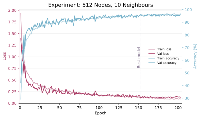
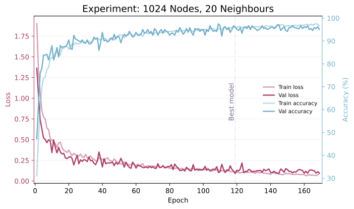
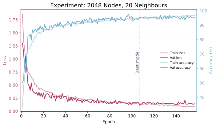
In this case study, we conduct three experiments:

Exp. 1: 512 nodes, with $k=10$
Exp. 2: 1024 nodes, with $k=20$
Exp. 3: 2048 nodes, with $k=20$

The code used for these experiments is available in this GitHub repository. All DGCNN models were trained with jitter noise of $\sigma=0.02$ and optimised using SGD with a momentum of $0.9$ and weight decay of $10^{-4}$ . The learning rate was decreased from $0.01$ to $0.0001$ over the course of training. Each model was trained for up to 250 epochs, with an early-stopping patience of 50 epochs. The Leaky ReLU slope was set to $0.2$ , the dropout rate to $0.5$ , and the batch-normalisation momentum to $0.1$ . With the exception of early stopping, these settings closely follow those used by Wang et al. (2019). The training histories for these three experiments are shown below:

Loss and accuracy curves for 512 points and k=10 — **Figure 5:** Training loss and accuracy curves for DGCNN experiments.

Loss and accuracy curves for 1024 points and k=20 — **Figure 5:** Training loss and accuracy curves for DGCNN experiments.

Results and Analysis

In the baseline and DGCNN experiments, the models were evaluated on the same held-out test split. The following sections present quantitative results, class-level errors, and t-SNE visualisations of the learned embeddings.

Quantitative

The table below shows the classification performance on the ModelNet10 test set (743 samples). The baseline model is compared against DGCNN models evaluated with three input configurations: 512 points with 10 edges, 1024 points with 20 edges, and 2048 points with 20 edges. Mean class accuracy, precision, and F1-score are macro-averaged over the 10 classes. Exp. 1, with its 512-10 point-edge configuration, achieves the best performance across all metrics. We also notice that performance drops across all metrics as we increase the number of points; this, alongside the results in Table 5 of Wang et al. (2019), suggests that the choice of the number of nodes and edges/k neighbours plays a crucial role in DGCNN performance. Thus, a hyperparameter sweep is needed before deciding on the best model.

Table 2. Quantitative results of all experiments.

Model	Overall Accuracy	Mean Class Accuracy (Recall)	Precision	F1-score
Baseline	0.92	0.89	0.90	0.89
Exp. 1: 512, 10	0.96	0.94	0.95	0.94
Exp. 2: 1024, 20	0.95	0.92	0.94	0.93
Exp. 3: 2048, 20	0.91	0.90	0.89	0.89

Figure 6 compares the overall test accuracy of the four configurations. The 512-point model with $k=10$ achieves the highest accuracy of $0.96$ , followed by the 1024-point model with $k=20$ at $0.95$ . The baseline achieves an accuracy of $0.92$ , while the 2048-point model with $k=20$ achieves the lowest accuracy of $0.91$ . These results show that increasing the number of input points does not necessarily improve classification performance.

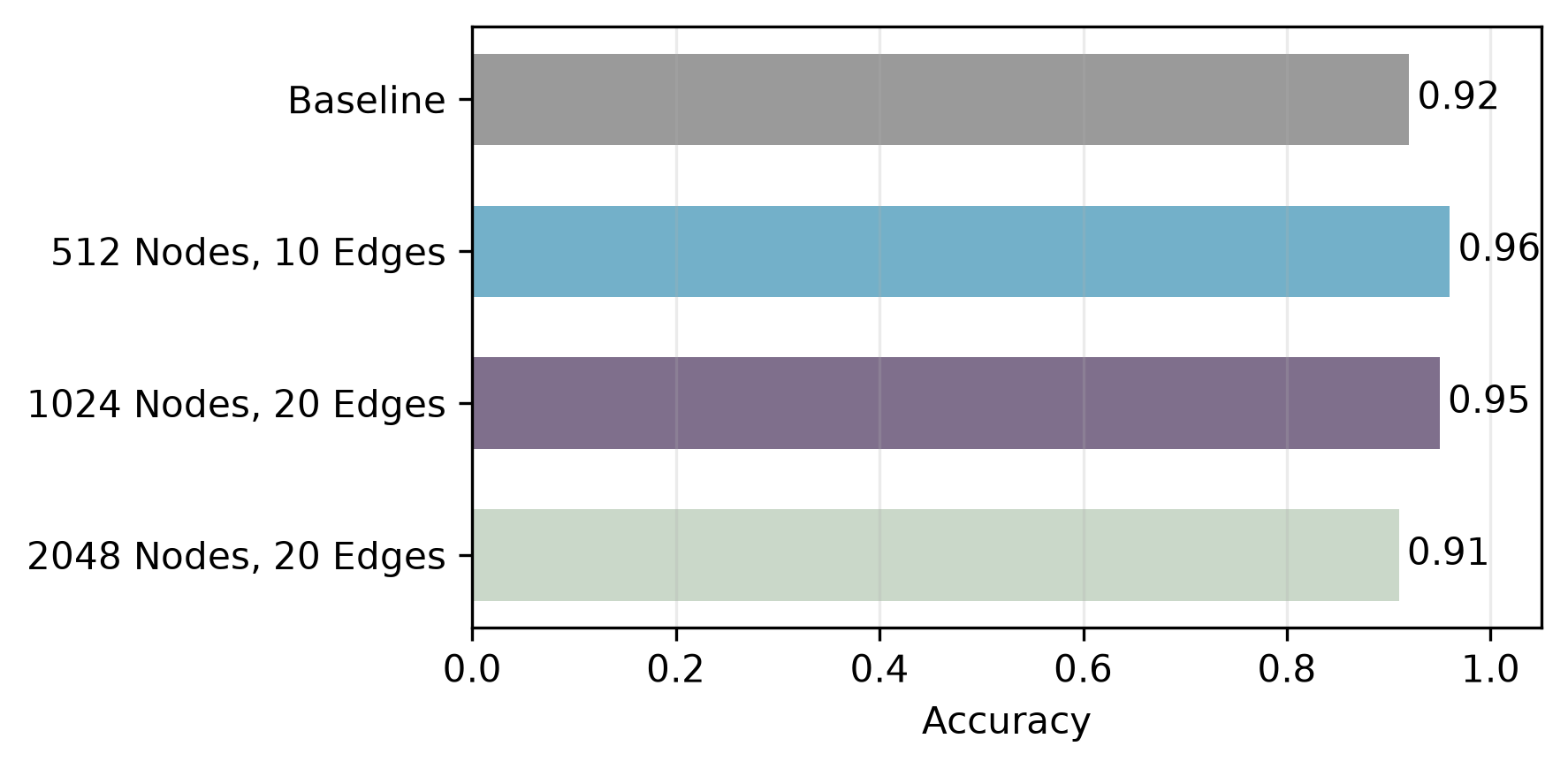
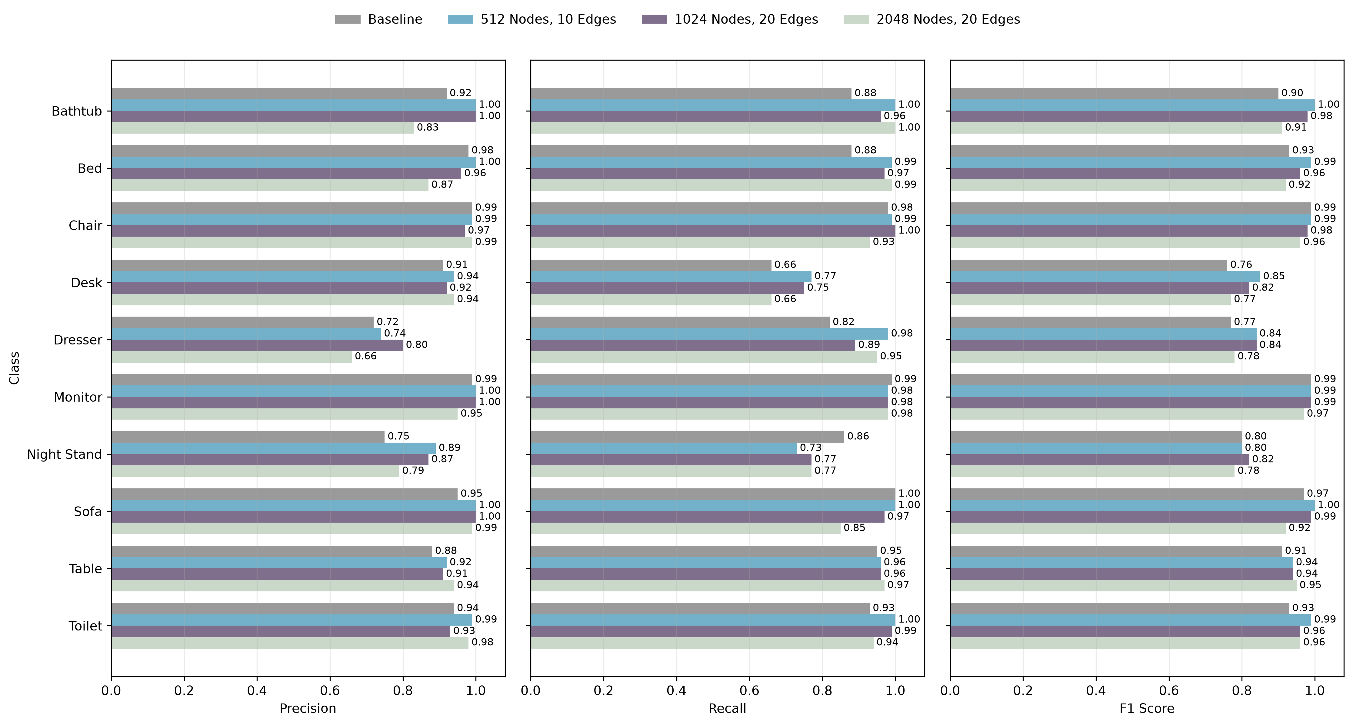
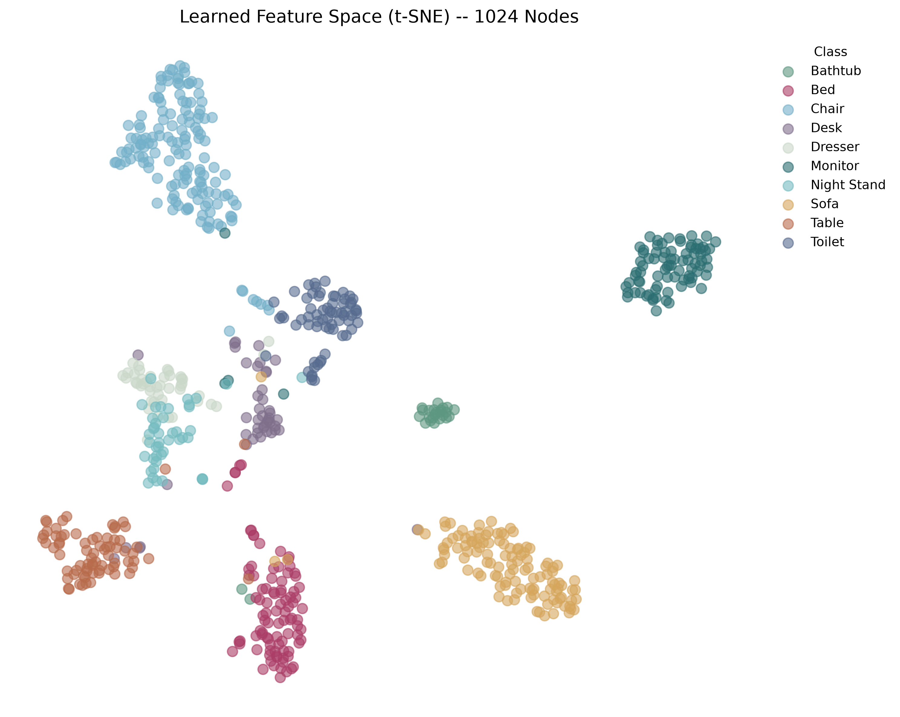
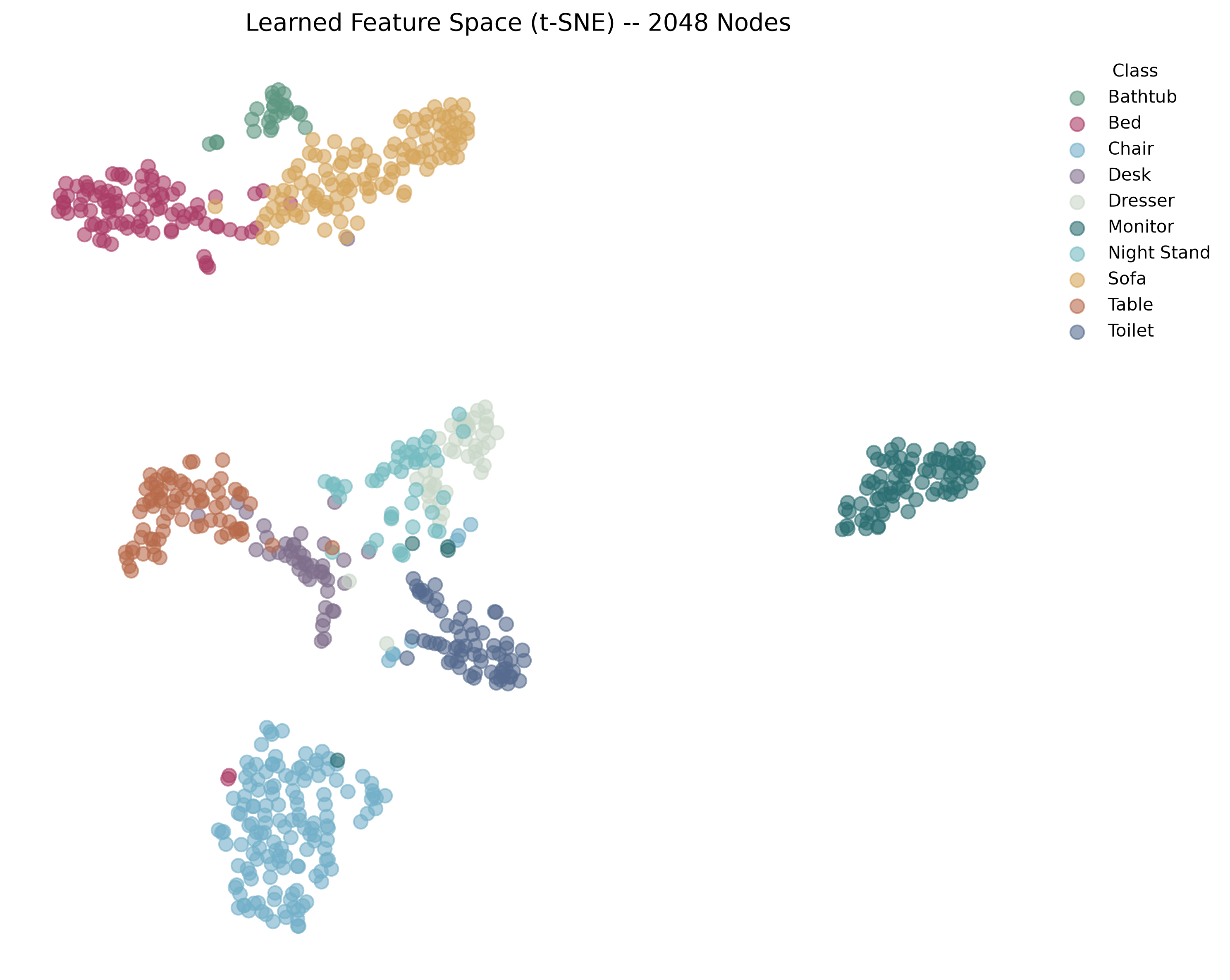
Overall test accuracy across DGCNN configurations — **Figure 6:** Overall test accuracy for the baseline and DGCNN models using 512 points with $k=10$, 1024 points with $k=20$, and 2048 points with $k=20$.

Figure 7 provides a class-level comparison of precision, recall, and F1-score. The 512-point model with $k=10$ generally achieves the most consistent performance across the ten classes, with particularly strong results for Bathtub, Bed, Chair, Monitor, Sofa, and Toilet. The largest differences between configurations appear for the more challenging classes, particularly Desk, Dresser, and Night Stand. For example, the 2048-point model achieves a recall of $0.66$ for Desk and a precision of $0.66$ for Dresser. This suggests that the differences in overall performance are largely driven by a small number of difficult classes rather than by a uniform change across all classes.

Per-class precision, recall, and F1-score across DGCNN configurations — **Figure 7:** Per-class precision, recall, and F1-score for the baseline and DGCNN models using 512 points with $k=10$, 1024 points with $k=20$, and 2048 points with $k=20$.

Qualitative

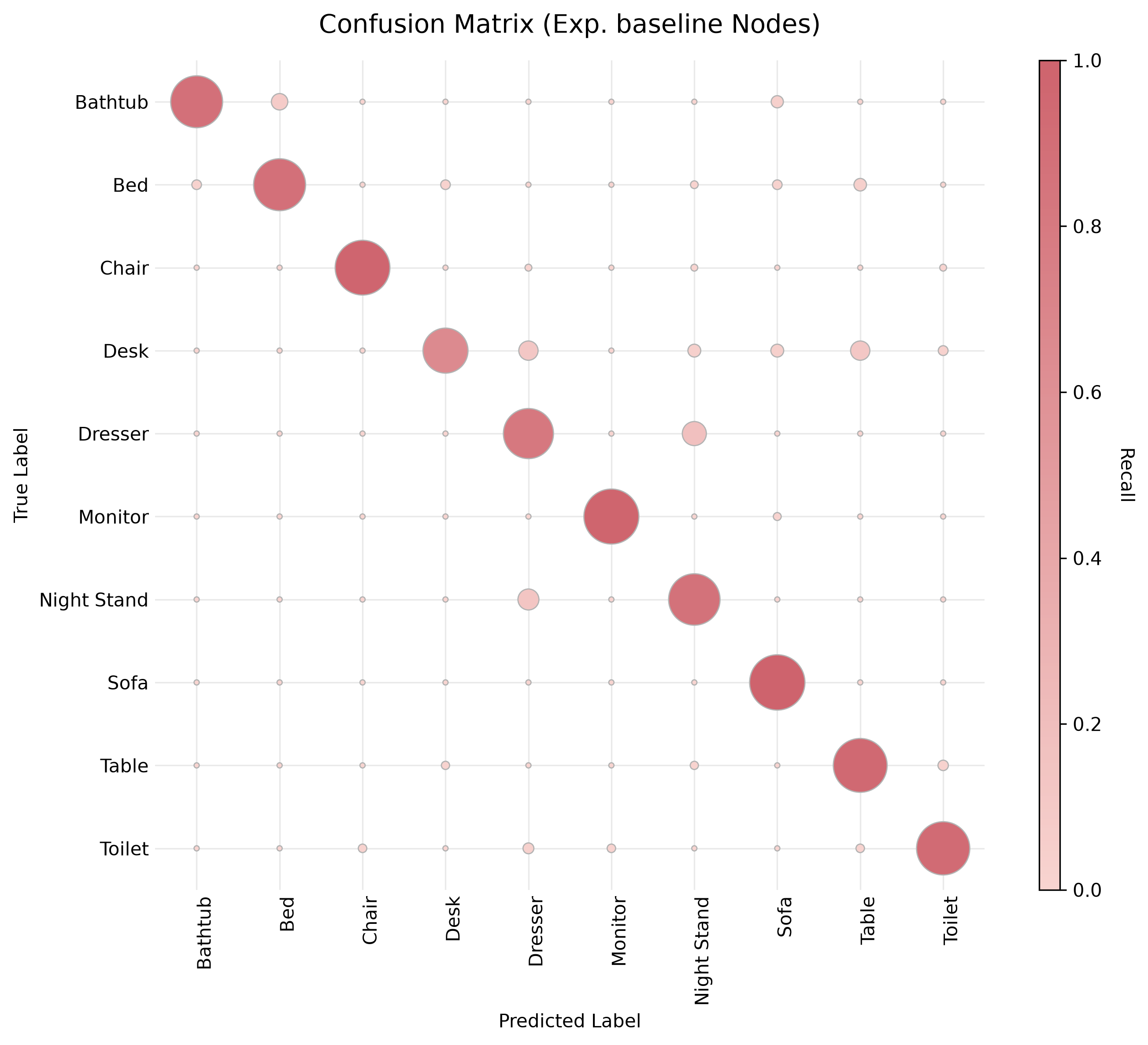
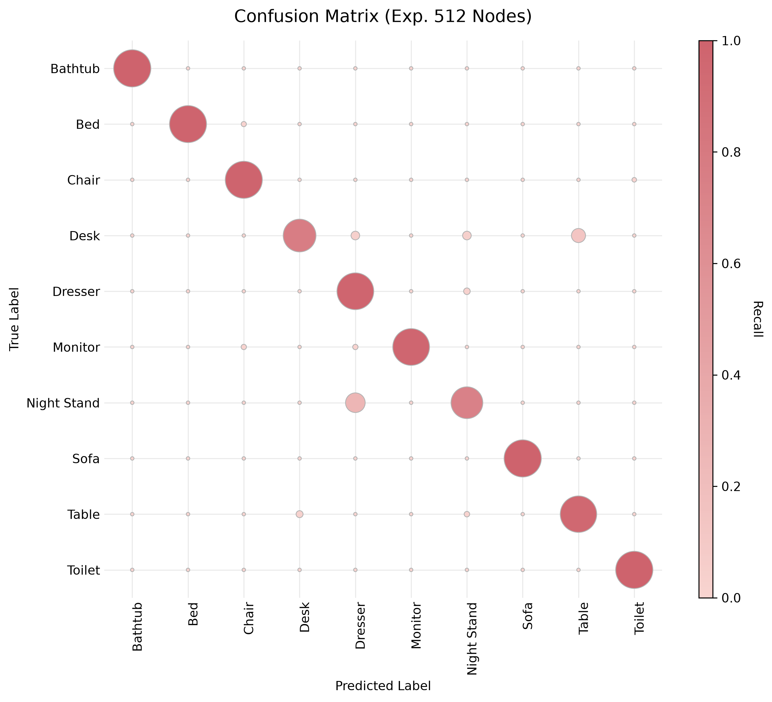
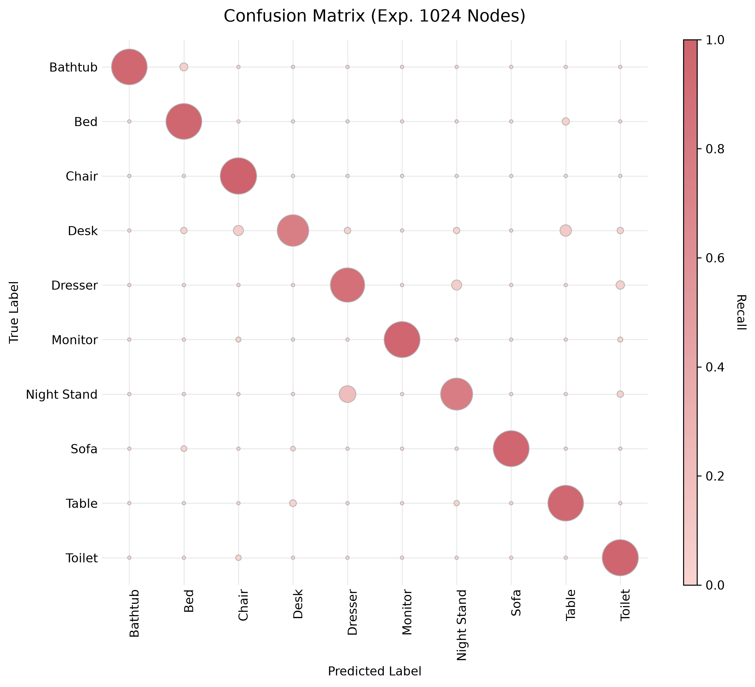
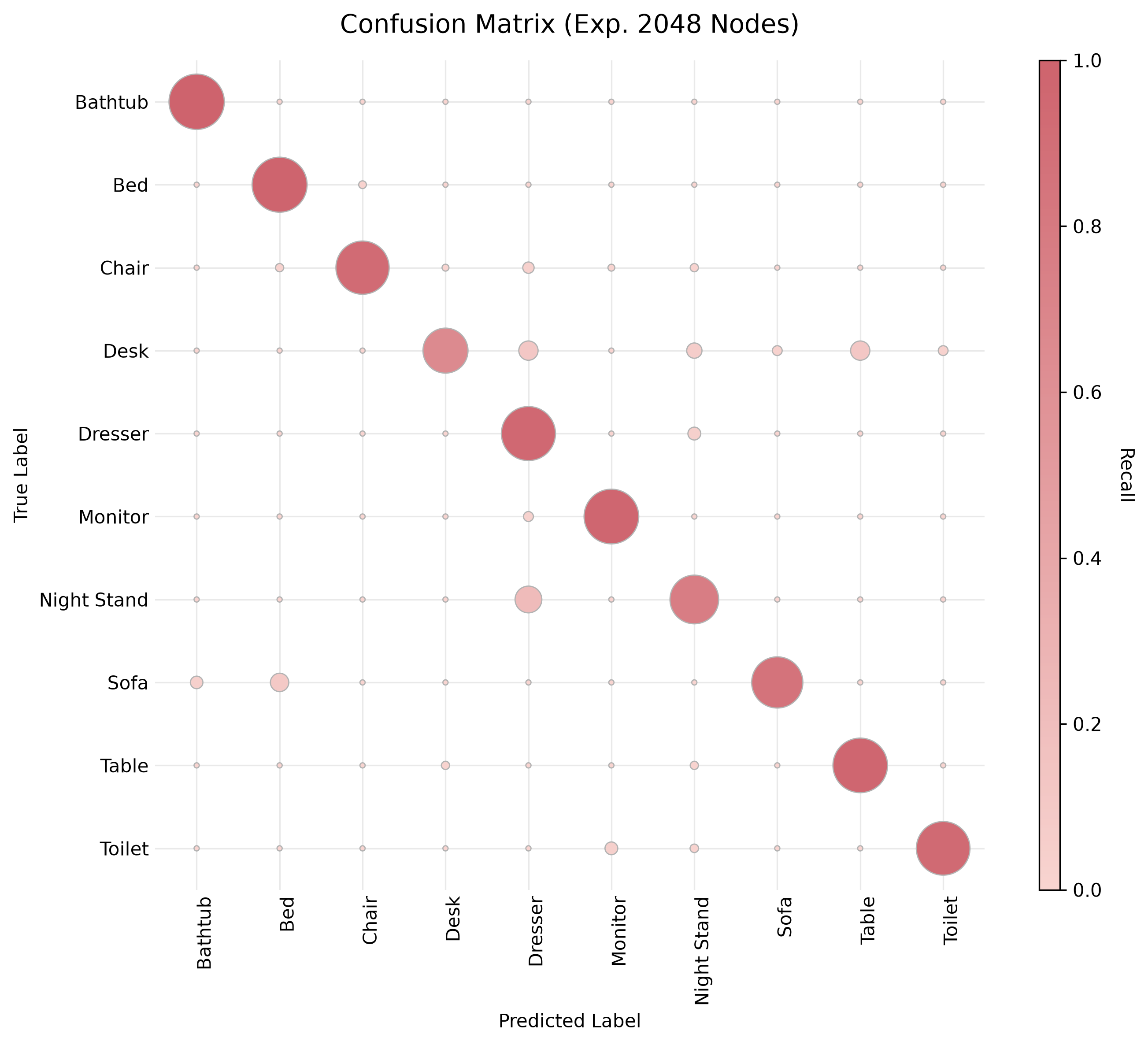
Figure 8 presents confusion matrices for the four experiments. It shows that all models struggled with Night Stand objects, frequently confusing them with Dresser objects. A similar pattern is observed for the Desk class, in which some objects are misclassified as Table objects. The consistency of these errors across different model configurations suggests an inherent challenge in distinguishing these classes within the dataset, which I investigate further using t-SNE analysis below.

Confusion matrix for the baseline DGCNN experiment — **Figure 8:** Normalised confusion matrices for the baseline DGCNN model (top left) and experiments using 512 (top right), 1024 (bottom left), and 2048 (bottom right) points per point cloud. Bubble size and colour intensity indicate the recall for each true–predicted class pair.

Confusion matrix for the DGCNN experiment with 512 points — **Figure 8:** Normalised confusion matrices for the baseline DGCNN model (top left) and experiments using 512 (top right), 1024 (bottom left), and 2048 (bottom right) points per point cloud. Bubble size and colour intensity indicate the recall for each true–predicted class pair.

t-SNE

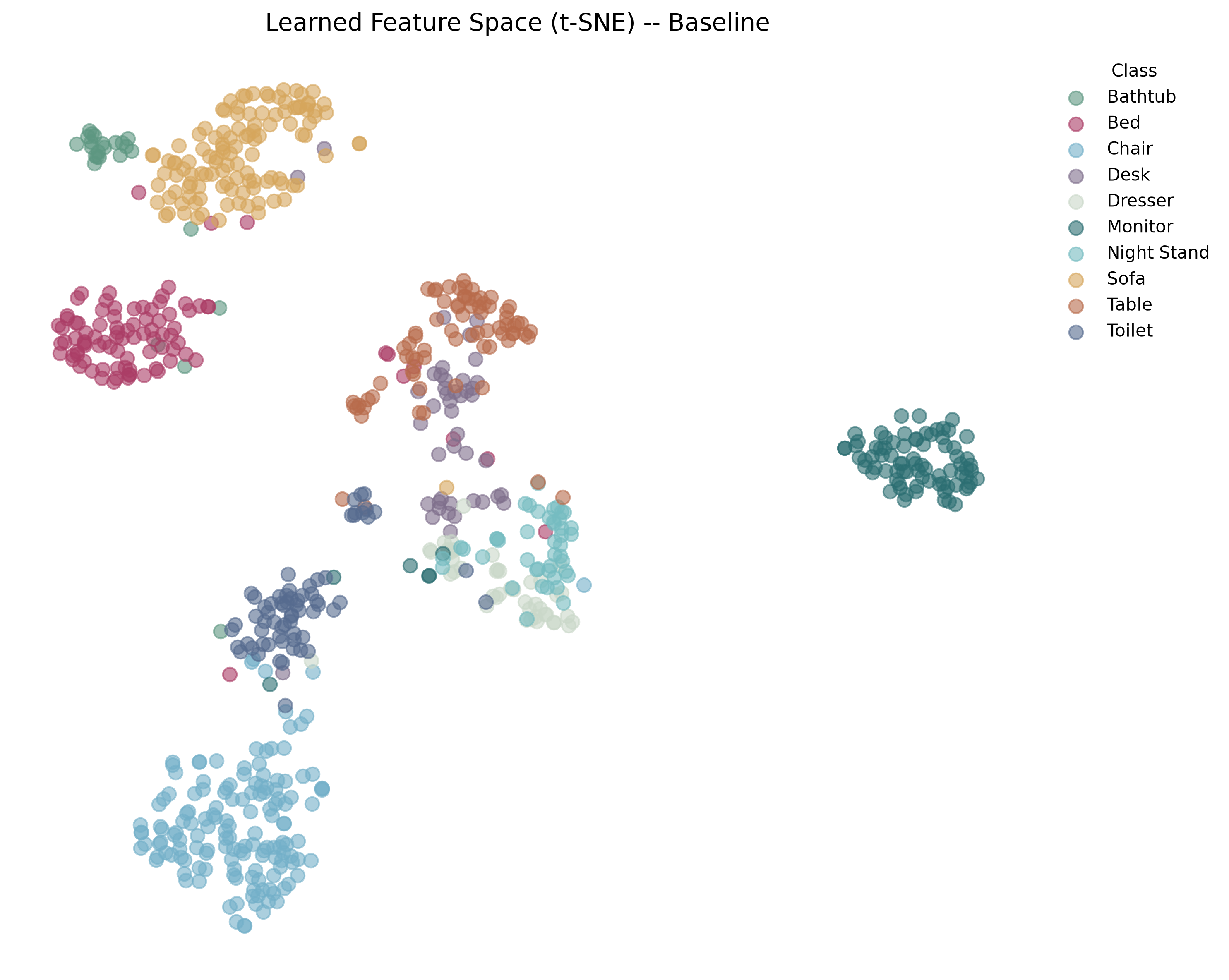
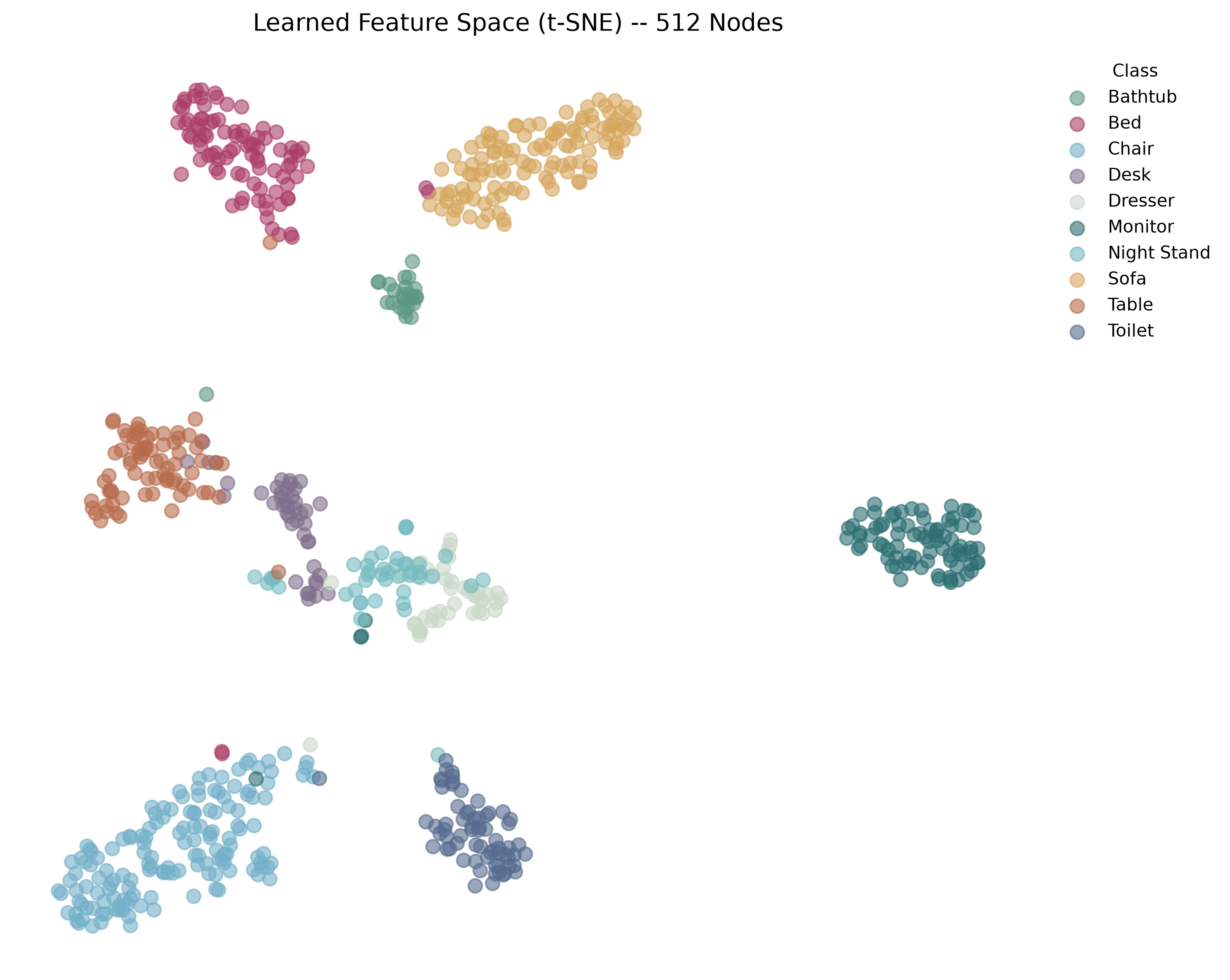
t-SNE (t-distributed stochastic neighbour embedding) is a non-linear dimensionality-reduction technique commonly used to visualise high-dimensional data in two dimensions. It aims to preserve local neighbourhood relationships, such that samples that are similar in the original feature space tend to appear close together in the resulting projection. In this case study, t-SNE is used to visualise the learned feature representations produced by the baseline and DGCNN models for the ModelNet10 test set. This allows us to qualitatively examine how well the models separate the different object classes in their latent spaces and to identify regions where classes overlap. In particular, the visualisation can help explain some of the confusion observed between similar classes, such as Desk, Dresser, Night Stand, and Table, by showing whether their learned representations occupy nearby or overlapping regions (the reader is encouraged to use the interactive graphs, which can be accessed by clicking on the relevant figure panel). Because t-SNE is primarily a visualisation method, the absolute distances and global arrangement of clusters should not be interpreted quantitatively; the focus is instead on the local structure and degree of class separation.

t-SNE projection for DGCNN using 512 points and k=10 — Figure 9: t-SNE projections of the learned feature spaces. Select a figure to open the interactive visualisation and inspect individual point clouds.

Conclusions and Limitations

It has been an interesting experience to work with point cloud data and reproduce the work presented in this paper. Many lessons were learnt. The most important ones concerned the nature of the updates made by the EdgeConv operation and working with 3D data. Point clouds remind me of the stars in the sky, except that stars are often studied in 6D (i.e. phase space) rather than 3D. Still, there is a unique opportunity to implement and adapt the method presented in this paper to study the nature of dark matter, as in Ma et al. (2025). I argue that using EdgeConv and DGCNN might be a better option than using the GCN operation. Previously, I highlighted this point:

It is worth highlighting that this entire operation is permutation invariant and partially translation invariant. In this way, the model learns not only how to extract local geometric features but also how to group points in a point cloud; therefore, distances in deeper layers carry semantic information over long distances in the original embedding.

I believe such a technique could have important applications in astrophysics and cosmology, particularly if it were paired with a physics objective (e.g. a loss function). It could help characterise the relationships between stars in a stellar stream (e.g. GD-1) in a high-dimensional feature space and identify perturbations in the stream. This could, in turn, help determine whether observed structures such as gaps and spurs are consistent with interactions with dark-matter subhaloes.

One limitation of this work is that it is not truly “dynamic”. In fact, the only dynamic aspects of this method are the evolution of the connections between nodes and the notion of a node’s “neighbour”. A truly dynamic graph would allow for the creation and annihilation of nodes and edges rather than having a fixed number of both (indeed, DGCNN changes “who your neighbours are”, not “how many neighbours you have”). Thus, an interesting next step would be to look for a method that does allow for the creation and annihilation of nodes and edges.

Another interesting application of this method is to use it to model the relationships between people and objects in a 2D or 3D scene. Such an approach could be integrated into a generative model to guide it in generating those images and the interactions they depict. For example, it could be used to model and discover complex relationships between objects and people in a 3D scene, and the generative model could be conditioned to maintain those relationships when generating the next scene.

Finally (this is a far-fetched idea), if a convolution operation is truly dynamic, allowing nodes and edges to be created and annihilated, a model using it could be effective for studying the interactions of quarks inside hadrons (i.e. baryons and mesons) or even in quark–gluon plasma. However, such a study must be constrained by physical laws and then tested thoroughly, since these laws might break down under such extreme conditions.

References

Bronstein, M.M., Bruna, J., Cohen, T. and Veličković, P., 2021. Geometric deep learning: Grids, groups, graphs, geodesics, and gauges. arXiv preprint arXiv:2104.13478.

Hamilton, W.L., 2020. Graph Representation Learning. Synthesis Lectures on Artificial Intelligence and Machine Learning, 14(3), pp. 1–159.

Ma, P.X., Rogers, K.K., Li, T.S., Hložek, R., Webb, J.J., Huang, R. and Meunier, J., 2025. Toward Characterizing Dark Matter Subhalo Perturbations in Stellar Streams with Graph Neural Networks. The Astrophysical Journal, 987(1), p. 96.

Wang, Y., Sun, Y., Liu, Z., Sarma, S.E., Bronstein, M.M. and Solomon, J.M., 2019. Dynamic graph CNN for learning on point clouds. ACM Transactions on Graphics (TOG), 38(5), pp. 1–12.

Continue reading

Explaining BERT model predictions with LIME for disaster tweets

April 12, 2024 5 min read

A case study on using BERT and LIME to classify disaster tweets, interpret model behavior, and communicate both the strengths and limits of the system.

Topics: NLP · BERT · LIME · explainability